How to Calculate the A-priori Power For a Path Model
Using semPower
by Arndt Regorz, MSc.
June 19, 2024
If you want to conduct a path analysis, e.g., with lavaan, AMOS, MPlus, jamovi, JASP, Stata, or other covariance-based SEM programs, you will need to determine the minimum sample size required.
While there are various rules of thumb for the minimum sample size when using SEM programs, these only try to indicate the sample size needed for a stable estimation. This does not necessarily mean that you have sufficient power to detect the hypothesized effects.
Therefore, an a-priori power calculation should be performed for sample size planning. This article shows how to use the semPower package for this purpose. A post-hoc power calculation is also possible with semPower, although its usefulness is quite controversial in the methodological literature.
Although semPower is an R package, its results can also be used for path analyses with other SEM programs. You do not need to learn to program with R; it is sufficient to install R and use the commands presented here - no prior experience with R is needed.
Content
- Overview of this tutorial
- Preparation for using semPower
- A-priori power for an entire path model
- Post-hoc power for an entire path model
- A-priori power for a specific path
- Checking if the model is correctly specified
- A-priori power for comparing two effects
- Post-hoc power for a specific effect
- Simulation-based power calculation
- Further power analyses
1. Overview of this Tutorial
In this tutorial, we will first consider power analyses for the entire model. This addresses the question: Does the specified path model fit the data?
We will then consider power calculations for specific effects. This addresses questions such as: Is the effect from variable A to variable B significant? Is the effect from variable A to variable C larger than the effect from variable B to variable C?
Finally, we will present some advanced options for power calculations in path analyses.
2. Preparation for Using semPower
For semPower as an R package, you first need R. There are numerous explanations on the internet and YouTube on how to install R.
You will also need the packages semPower and lavaan. These need to be installed once, with:
install.packages("semPower")
install.packages("lavaan")
And in each R session in which you want to work with semPower, load these packages with the commands:
library(semPower)
library(lavaan)
Power for an Entire Path Model
3. A-priori Power for an Entire Path Model
Path analyses are model-testing procedures used to estimate the degree of agreement between a theoretical model and empirically collected data.
Let's take an example in which you want to test this model:
Figure 1
Example Path Model
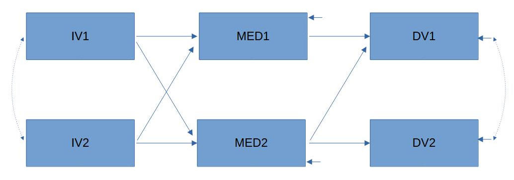
How large does the sample need to be to detect a significant discrepancy between your data and the model?
To perform an a-priori power calculation for a full model, you need the degrees of freedom of the model. These can either be calculated manually or - if you are working with lavaan - automatically calculated from your model definition using a function from the semPower package.
Manually calculated, you can get the degrees of freedom as the difference between the number of empirical pieces of information and the number of parameters to be estimated.
The number of empirical pieces of information is derived from the formula k * (k + 1) / 2 for k measured variables, which is 6 * 7 / 2 = 21 for this example
The number of parameters to be estimated consists in this example of 6 variances of the measured variables (or their disturbances), 7 directed effects, and 2 covariances, totaling 15.
This leaves 21 - 15 = 6 degrees of freedom for this model.
If you want to estimate the model with lavaan, you can calculate this value directly from the lavaan model code. The example path model can be specified with the following code:
path1 <- '
MED1 ~ IV1 + IV2
MED2 ~ IV1 + IV2
DV1 ~ MED1 + MED2
DV2 ~ MED2
IV1~~IV2
DV1~~DV2
'
Using the `semPower.getDf()` function from the semPower module, you can determine the degrees of freedom directly with this model code:
semPower.getDf(path1)
The result will be 6 degrees of freedom.
After obtaining the degrees of freedom of the model, we can now perform the a-priori power calculation.
To do this, we need to specify the smallest effect we want to detect with a set power. There are various effect size measures for this. The most straightforward is probably the fit index RMSEA. With the following code, you can use the semPower.aPriori() function to determine the necessary sample size to detect a discrepancy between the model and the data of at least RMSEA = .06 with a power of .80.
path_full_1 <- semPower.aPriori(effect = 0.06,
effect.measure = 'RMSEA',
alpha = .05,
power = .80,
df = 6)
summary(path_full_1)
The result is:
semPower: A priori power analysis
F0 0.021600
RMSEA 0.060000
Mc 0.989258
df 6
Required Num Observations 631
Critical Chi-Square 12.59158
NCP 13.60800
Alpha 0.050000
Beta 0.200559
Power (1 - Beta) 0.799441
Implied Alpha/Beta Ratio 0.249303
Here, an extremely large sample size of 631 is indicated. This is because for models with few degrees of freedom the RMSEA can become very high with even slight discrepancies between the data and the model, and therefore RMSEA often yields misleading results for models with few degrees of freedom (e.g. with df < 10).
Hence, for a model with so few degrees of freedom, it is better to use another effect size measure, such as the fit index AGFI. For a good fit, this should be above .90.
To repeat the power calculation using AGFI instead of RMSEA, we need to add an additional parameter to the function call: the number of measured variables in the model (p), which in our case is 6.
path_full_2 <- semPower.aPriori(effect = 0.90,
effect.measure = 'AGFI',
alpha = .05,
power = .80,
df = 6,
p = 6)
summary(path_full_2)
The result now shows a much more realistic sample size of 157.
In addition to the above output, a graph for the power is also provided, but in my opinion, it does not add any significant relevant information.
4. Post-hoc Power for an Entire Path Model
If you want to calculate the achieved power retrospectively, you can use the semPower.postHoc() function by entering the actually achieved effect size (e.g., AGFI or RMSEA) and the actual sample size realized. The other parameters remain the same as for the a-priori power calculation.
path_full_3 <- semPower.postHoc(effect = 0.92,
effect.measure = 'AGFI',
alpha = .05,
N = 120,
df = 6,
p = 6)
summary(path_full_3)
In this example, the empirically achieved power is 0.5518.
Power for Specific Effects
5. A-priori Power for a Specific Path
Usually, hypotheses are made for specific paths. With semPower, one can also calculate the sample size required to achieve a predetermined power for testing a specific path.
(If there are multiple hypotheses for several paths of the path model, a power calculation is conducted for each hypothesis, and then the largest resulting sample size is used.)
When we want to calculate the power for specific paths, we first need assumptions about the empirical relationships between the model variables in reality. The difficult part is, of course, getting to realistic assumptions for all paths and correlations, ideally based on published literature.
As soon as we have made assumptions we can input those into semPower. For this, we create two matrices: a matrix of (standardized) effects, i.e., the Betas, and a correlation matrix Psi.
First, the Beta matrix:
Beta1 <- matrix(c(
c(.00, .00, .00, .00, .00, .00), # IV1
c(.00, .00, .00, .00, .00, .00), # IV2
c(.30, .30, .00, .00, .00, .00), # MED1 = 0.3 * IV1 + 0.3 * IV2
c(.10, .50, .00, .00, .00, .00), # MED2 = 0.1 * IV1 + 0.5 * IV2
c(.00, .00, .30, .10, .00, .00), # DV1 = 0.3 * MED1 + 0.1 * MED2
c(.00, .00, .00, .30, .00, .00) # DV2 = 0.3 * MED2
), byrow = TRUE, ncol = 6)
This matrix has as many rows and columns as there are variables in the model.
The entries in the individual rows are the effects on the respective nth variable. The entries in the columns are the effects from the respective nth variable.
E.g., the 2nd value in the 3rd row is the effect from the 2nd variable (IV2) on the third variable (MED1).
The order of the variables should be from left to right, starting with the independent variables in the path diagram, then the mediators (possibly in several layers), and then the dependent variables.
If, instead, you had a path model with eight measured variables instead, you would have eight rows of data, with eight entries in each row, and in the end, ncol = 8.
Besides the directed effects, we also need assumptions about the correlations between the model variables (correlations for the exogenous variables IV1 and IV2, residual correlations for the endogeneous variables MED1, MED2, DV1, DV2).
Psi1 <- matrix(c(
c( 1, .30, .00, .00, .00, .00), # IV1
c(.30, 1, .00, .00, .00, .00), # IV2
c(.00, .00, 1, .00, .00, .00), # MED1
c(.00, .00, .00, 1, .00, .00), # MED2
c(.00, .00, .00, .00, 1, .20), # DV1
c(.00, .00, .00, .00, .20, 1) # DV2
), byrow = TRUE, ncol = 6)
There is a 1 in the main diagonal. Additionally, correlations between any two variables (or their disturbances) are entered twice, above the diagonal and below. The order of the variables is the same as above in the Beta matrix.
In this example, there are two correlations:
IV1-IV2: .30
.DV1-.DV2: .20
With these preparations, the actual a-priori power analysis can be conducted using the function semPower.powerPath().
path_path1 <- semPower.powerPath(type = 'a-priori',
Beta = Beta1,
Psi = Psi1,
nullEffect = 'beta=0',
nullWhich = c(3, 1),
Lambda = diag(6), # number of variables
alpha = .05,
power = .80)
summary(path_path1)
First, the type ('a-priori') is specified.
The two matrices Beta1 and Psi1 created above are passed.
Then it is specified that the power should be calculated to see if a specific effect is significantly different from zero (nullEffect = 'beta=0').
Next, it specifies which specific effect in the hypothesis is to be tested (nullWhich = c(3, 1)), in this example, the effect from the third row and first column of the Beta1 matrix, i.e., the effect on the third variable (MED1) from the first variable (IV1) of the matrix.
The entry at Lambda is intended for the loadings (this function can also be used to perform power calculations for full SEM models with latent variables). In the path model, there are no loadings (more precisely: each construct has an indicator with a loading of 1). Here, you simply enter the number of model variables in diag(...).
Finally, alpha and the desired power are specified.
As a result, we obtain:
semPower: A priori power analysis
F0 0.101581
RMSEA 0.318717
Mc 0.950478
df 1
Required Num Observations 79
Critical Chi-Square 3.841459
NCP 7.923282
Alpha 0.050000
Beta 0.196311
Power (1 - Beta) 0.803689
Implied Alpha/Beta Ratio 0.254698
A sample size of 79 is needed to achieve a power of .80 for testing the effect of IV1 on MED1, assuming the specified model effects and correlations.
6. Checking if Model is Correctly Specified
To ensure that the model relationships have been specified as intended, one can output the resulting models (the H1 model with the expected relationships and the H0 model with one path set to zero).
p_calc <- path_path1
h1_model <- lavaan::sem(p_calc$modelH1, sample.cov = p_calc$Sigma,
sample.nobs = p_calc$requiredN, sample.cov.rescale = FALSE)
h0_model <- lavaan::sem(p_calc$modelH0, sample.cov = p_calc$Sigma,
sample.nobs = p_calc$requiredN, sample.cov.rescale = FALSE)
summary(h1_model, standardized = T)
summary(h0_model, standardized = T)
You don't need to understand this code in detail. What is important for you is the first line. You need to replace path_path1 with the name of your power analysis result. The rest of the code remains the same.
As a result, you will get a lavaan output for your H1 model and your H0 model. Here, you can check if the models have been set up as desired. For the H0 model, note that usually not only the specific effect tested differs from the H1 model, but also other effects might differ. This is normal since in a path model, all estimates are interrelated, and setting one effect to zero can trigger changes in the estimation results of other effects.
7. A-priori Power for Comparing Two Effects
If your hypothesis is that one effect is greater than another, you can also perform a power calculation for that.
path_path2 <- semPower.powerPath(type = 'a-priori',
Beta = Beta1,
Psi = Psi1,
nullEffect = 'betaX = betaZ',
nullWhich = list(c(5, 3), c(5, 4)),
Lambda = diag(6), # number of variables
alpha = .05,
power = .80)
summary(path_path2)
Again, we need a matrix of effects (Beta) and a matrix of correlations (Psi). Here I use the same matrices from above.
The null effect is now defined differently ('betaX = betaZ'), and nullWhich now passes a list of two effects: the two effects we want to compare in the hypothesis. Here they are the effects from the 5th row and 3rd column (MED1-DV1) and from the 5th row and 4th column (MED2-DV1) of the Beta matrix. We want to test if MED1 has a significantly stronger/weaker influence on DV1 than MED2. The other specifications remain the same.
In the example, we would get a required sample size of 448.
8. Post-hoc Power for a Specific Effect
In addition to an a-priori power analysis, a post-hoc power calculation can also be performed.
First, we create the matrices of the actually estimated beta weights and correlations:
Beta2 <- matrix(c(
c(.00, .00, .00, .00, .00, .00), # IV1
c(.00, .00, .00, .00, .00, .00), # IV2
c(.25, .35, .00, .00, .00, .00), # MED1
c(.15, .55, .00, .00, .00, .00), # MED2
c(-.05, .05, .30, .10, .00, .00), # DV1
c(.10, .00, .00, .30, .00, .00) # DV2
), byrow = TRUE, ncol = 6)
Psi2 <- matrix(c(
c( 1, .35, .00, .00, .00, .00), # IV1
c(.35, 1, .00, .00, .00, .00), # IV2
c(.00, .00, 1, .05, .00, .00), # MED1
c(.00, .00, .05, 1, .00, .00), # MED2
c(.00, .00, .00, .00, 1, .25), # DV1
c(.00, .00, .00, .00, .25, 1) # DV2
), byrow = TRUE, ncol = 6)
Then follows the actual power calculation.
path_path3 <- semPower.powerPath(type = 'post-hoc',
Beta = Beta2,
Psi = Psi2,
nullEffect = 'beta=0',
nullWhich = c(3, 1),
Lambda = diag(6), # number of variables
alpha = .05,
N = 150)
summary(path_path3)
Here, the type is 'post-hoc'. Additionally, instead of specifying the desired power, the achieved sample size N is provided. You are already familiar with the rest of the parameters from above.
As a result, we would obtain an empirically achieved power of .89885.
9. Simulation-based Power Calculation
The previous power calculations were analytical, based on the assumed distributions. Instead, a simulation-based power calculation can also be performed with semPower.
set.seed(12345)
path_path4 <- semPower.powerPath(type = 'a-priori',
Beta = Beta1,
Psi = Psi1,
nullEffect = 'beta=0',
nullWhich = c(3, 1),
Lambda = diag(6), # number of variables
alpha = .05,
power = .80,
simulatedPower = TRUE,
simOptions = list(nReplications = 500))
summary(path_path4)
Newly added is the specification of a seed value at the top as well as the last two lines of the semPower.powerPath function call, which ensure that a simulated power calculation is now performed (the number of replications should probably be significantly higher than 500 in reality, though the calculation would then take much longer).
This is only a very simple example of a simulated power calculation. With simulations you can calculate the power for more difficult questions, too, for example if you expect missing data, non-normal distributions, etc. For that please refer to the documentation of the semPower module.
10. Advanced Power Analyses
There are numerous other options for conducting power calculations in path models. These will only be briefly mentioned here so that you know they exist. Example code can be found in the documentation of the semPower module.
Path Comparison in Multi-Group Models
One can also calculate the power for a multi-group path model where one wants to test if an effect significantly differs between two groups. For this, the function semPower.powerPath() can be used with the null effect defined as 'betaA = betaB'. In this case, two matrices of betas and correlations need to be created (one for each group). For details, see the semPower documentation.
Indirect Effects (Mediation)
In path models, there is often an interest in indirect effects (mediations). To test the power for an indirect effect, there is a special function in semPower, the semPower.powerMediation() function. The main difference from the semPower.powerPath() function is that here, the indirect effect for which power is to be calculated must be specified. For details, see the semPower documentation.
However, in this case you should only use the simulation option for the power analysis, since I believe the analytical power calculation can result in sample sizes that are too small for a mediation analysis (especially if a-path and b-path have similar effect sizes).
Cross-Lagged Panel Models (CLPM)
If one wants to estimate a Cross-Lagged Panel Model, one can use the procedure described above for power calculation. However, one can also use a special function of semPower, the semPower.powerCLPM() function. This saves time and reduces the risk of errors in input. For details, see the semPower documentation.
Random-Intercept Cross-Lagged Panel Models (RI-CLPM)
Random-Intercept Cross-Lagged Panel Models have established themselves in recent years as an alternative to ordinary CLPM, offering conceptual advantages in certain situations. For this, there is also a special function, semPower.powerRICLPM(). For details, see the semPower documentation.
Other Special Functions
There are further special functions in semPower that might be relevant for models with manifest variables:
- semPower.powerARMA() for ARMA models (autoregressive models with moving averages)
- semPower.powerAutoreg() for autoregressive models
- semPower.powerLGCM() for Latent Growth Curve Models
For details, see the semPower documentation.
References
Moshagen, M., & Bader, M. (2023). Package ‘semPower’ (Version 2.1.0). CRAN. https://cran.r-project.org/web/packages/semPower/semPower.pdf
Moshagen, M., & Bader, M. (2023). semPower: General power analysis for structural equation models. Behavior Research Methods, Advance online publication. https://doi.org/10.3758/s13428-023-02254-7
Citation
Regorz, A. (2024, June 19). How to calculate the a-priori power for a path model: Using semPower. Regorz Statistik. https://www.regorz-statistik.de/blog/power_path_analysis_sempower.html