Exploratory Structural Equation Modeling (ESEM) With Lavaan

by Arndt Regorz, MSc.
March 4, 2025

Exploratory Structural Equation Modeling (ESEM) combines the best of two worlds: Exploratory factor analysis (EFA) and structural equation modeling (SEM). In an ESEM model you can substitute one or more measurement models for latent variables with EFAs.

This can give you among others the following advantages:

More robust than traditional SEM and CFA
Better fitting models
Less risks of biased correlations or directional paths

This blogpost will show you how to implement this approach with the lavaan package in r.

Example 1

As an example, let us say we want to investigate the relationship between stress, happiness and productivity. Our theory is that stress influences (here decreases) happiness and happiness increases productivity.

And let us say we have a three dimensional measurement instrument for stress (e.g. stress, depression, and anxiety) and a two-dimensional measurement instrument for happiness (e.g., positive affect and negative affect).

A conventional SEM could look like the model in figure 1.

Figure 1 Conventional SEM Model

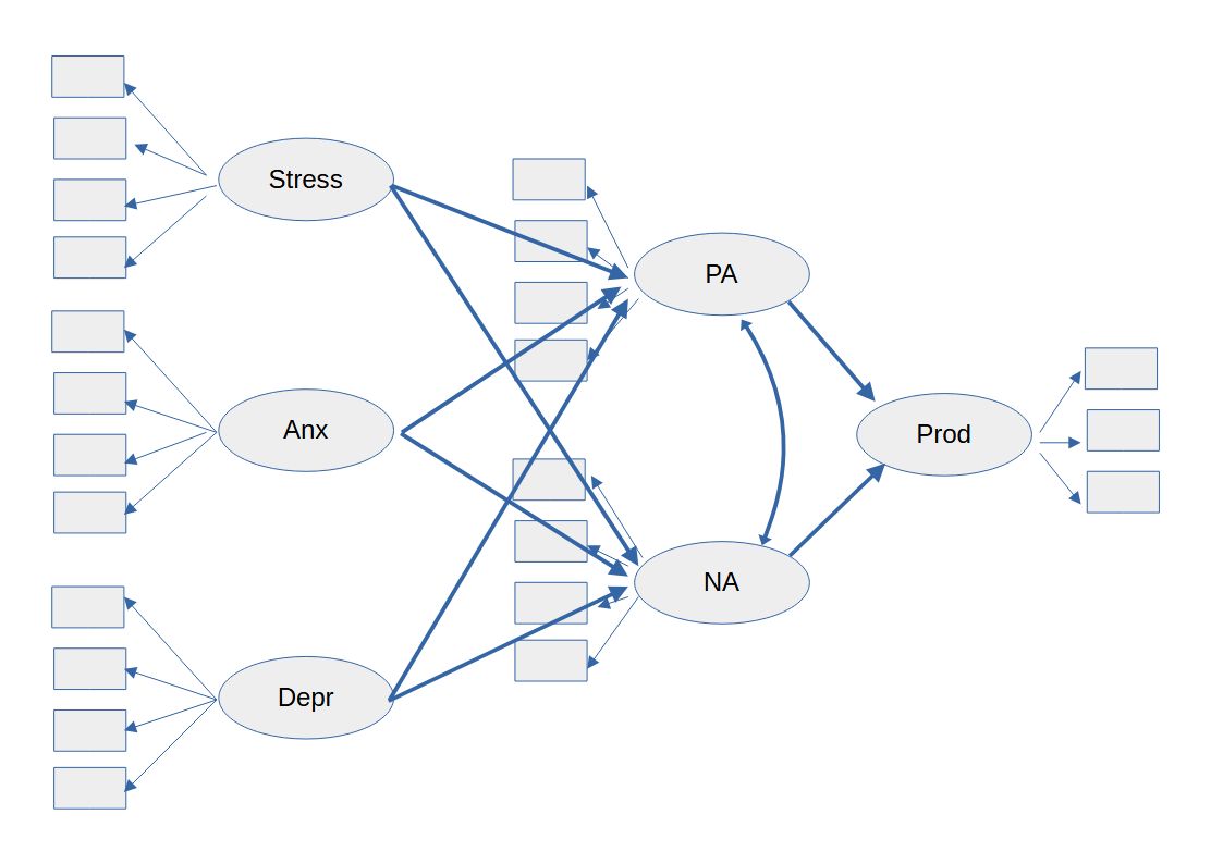
But often a model like this will not achieve a close fit because multidimensional constructs often have cross loadings.

Instead of the conventional SEM model we could use ESEM, using one EFA for stress and a second EFA for happiness, see figure 2.

Figure 2 ESEM Model

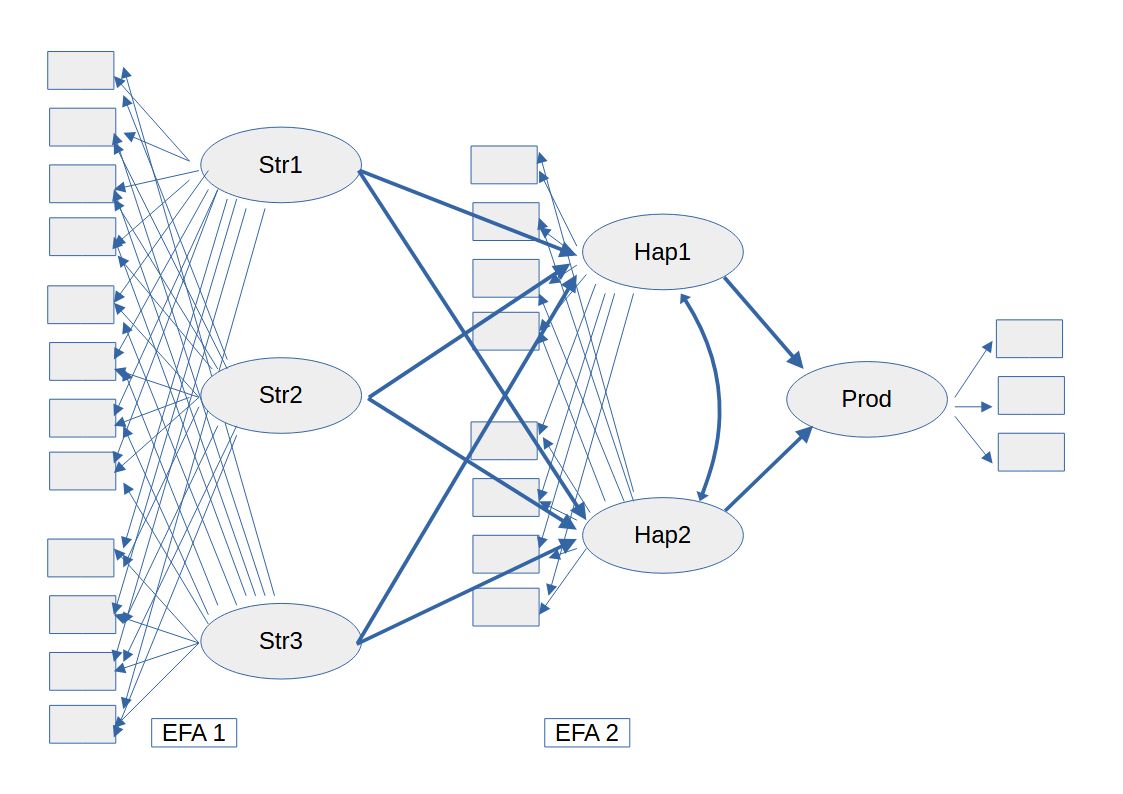
ESEM model (exploratory structural equation modeling

Note. As far as I know there is no canonical notation for the figure of an ESEM model. The graph above is just the way I like to plot an ESEM model.

This would be the R code for this ESEM model:

example_model <- '

# EFA 1
efa("efa1") * stress_1 +
efa("efa1") * stress_2 +
efa("efa1") * stress_3 =~ item1_1 + item1_2 + item1_3 +
item1_4 + item1_5 + item1_6 +
item1_7 + item1_8 + item1_9 +
item1_10 + item1_11 + item1_12

# EFA 2
efa("efa2") * happy_1 +
efa("efa2") * happy_2 =~ item2_1 + item2_2 + item2_3 +
item2_4 + item2_5 + item2_6 +
item2_7 + item2_8

# CFA
productivity =~ item3_1 + item3_2 + item3_3

# Regressions
happy_1 ~ stress_1 + stress_2 + stress_3
happy_2 ~ stress_1 + stress_2 + stress_3
productivity ~ happy_1 + happy_2

# Covariances
happy_1 ~~ happy_2 '

In this code there are many parts that you will already know from conventional SEM models in lavaan: The definition of the measurement model for productivity, the definition of the regression paths and of the covariances. New is the definition of the two EFA blocks. Let us look at those in more detail.

Here, a three factor EFA is specified with factor (latent variable) names stress_1, stress_2, and stress_3. Please note that we can’t give more specific names to the three factors even though we know that those should be, based on our theory, stress, depression, and anxiety. That is because we can’t know in advance which factor of the three factor EFA will get the stress items assigned to it, which factor will get the depression items and which will get the anxiety items. Only after having estimated the model can we deduce from the factor loading pattern which factor (stress_1 to stress_3) has which meaning.

In front of the factor names is the keyword efa, followed by a parenthesis with the name of the EFA block in quotation marks. For all factors that go into one EFA the name of the block has to be the same, here I have named the block “efa1” (you could choose a different name without changing the results).

The factors, in this example three, are linked by the plus sign. And after the last factor follows the factor loading operator =~ and the names of the items that go into the efa.

In plain English the code above says: Calculate a three-factor EFA, use the items item1_1 to Item1_12, and name the three factors stress_1, stress_2 and stress_3.

By default, lavaan uses an oblique rotation for the EFA (i.e., the factors are allowed to be correlated).

The block EFA2 works the same, just that there we extract only two factors.

The estimation of a model like this works just as a normal SEM estimation in lavaan:

model_fit1 <- sem(data = my_data_set,
model = example_model)

If you want to change the rotation method for the EFA, you can do that as part of the model estimation. For example this would be the code for an ESEM with the orthogonal Varimax rotation method:

model_fit1 <- sem(data = my_data_set,
model = example_model,
rotation ="varimax"))

You can find a list of all available rotation methods using the help function:

?efa

However, in most cases I would not change the rotation method from the default oblique rotation.

And you can display the results with the summary function.

summary(model_fit1,
fit.measures = T,
standardized = T)

Example 2

After the theoretical example above, here we will look at an example with real data. It is based on the dataset DASS, a very large dataset (nearly 40,000 observations) investigating the three dimensional stress inventory Depression Anxiety Stress Scales.

You can download the data at openpsychometrics.org: https://openpsychometrics.org/_rawdata/

For our example we want to investigate whether the personality dimension extraversion is able to predict the different dimensions of stress. (In the dataset, extraversion is measured with only two items. For the example a scale value was calculated from those two items, one of which had to be recoded first.)

library(lavaan)

First, we calculate the score on the extraversion short scale:

# Calculate Extraversion Score
DASS$TIPI6r <- 8 - DASS$TIPI6 # recode inverted item
items_extrav <- data.frame(DASS$TIPI1, DASS$TIPI6r)
DASS$extrav <- rowMeans(items_extrav, na.rm=TRUE)

Classical SEM Model

As a comparison for the later estimation of the ESEM model, let us first run a conventional SEM model:

# Classical SEM

model1 <- '
dep =~ Q3A + Q5A + Q10A + Q13A + Q16A +
Q17A + Q21A
stress =~ Q1A + Q6A + Q8A + Q11A +
Q12A + Q14A + Q18A
anx =~ Q2A + Q4A + Q7A + Q9A + Q15A +
Q19A + Q20A
dep ~ extrav
stress ~ extrav
anx ~ extrav
'

model_fit1 <- sem(data = DASS,
model = model1)
summary(model_fit1,
fit.measures = T,
standardized = T)

modindices(model_fit1,
minimum.value = 10,
sort=TRUE)

The chi square value for this model was very high (25398.58) and significant, but that was to be expected with a sample size of 39,775.

The main fit indices showed a moderately good fit, CFI = .943, RMSEA = .056, and SRMR = .037.

Here are the first eight lines of the modification indices:

lhs op rhs mi epc sepc.lv sepc.all sepc.nox
92 anx =~ Q12A 4046.905 1.296 0.740 0.694 0.694
216 Q1A ~~ Q11A 2381.257 0.135 0.135 0.311 0.311
77 stress =~ Q9A 1566.810 0.606 0.481 0.450 0.450
185 Q17A ~~ Q21A 1499.011 0.109 0.109 0.240 0.240
80 stress =~ Q20A 1350.385 0.578 0.459 0.411 0.411
70 stress =~ Q13A 1326.413 0.312 0.248 0.231 0.231
91 anx =~ Q11A 1278.270 -0.670 -0.383 -0.365 -0.365
240 Q8A ~~ Q12A 1219.023 0.117 0.117 0.197 0.197

In addition to some error covariances we can see a number of possible cross loadings which was to be expected in a multidimensional measurement instrument like this. (Please note that the absolute value of the modification index in the column “mi” is not that helpful in a model with such a large sample size. Here, I would concentrate on the column “sepc.all”, standardized expected parameter change.)

ESEM Model

For that reason, now we would like to run an ESEM model with the same data, specifying a three factor EFA for the items from the stress questionnaire.

Here is the model specification:

# ESEM

esem.model <- '
# EFA
efa("efa1") * dsa1 +
efa("efa1") * dsa2 +
efa("efa1") * dsa3 =~ Q3A + Q5A + Q10A + Q13A + Q16A +
Q17A + Q21A +
Q1A + Q6A + Q8A + Q11A +
Q12A + Q14A + Q18A +
Q2A + Q4A + Q7A + Q9A + Q15A +
Q19A + Q20A

# Regressions
dsa1 ~ extrav
dsa2 ~ extrav
dsa3 ~ extrav
'

We can run this model like any other SEM model:

model_fit2 <- sem(data = DASS,
model = esem.model)

summary(model_fit2,
fit.measures = T,
standardized = T)

Comparing the model fit we can see that the fit indices have been improved:
CFI .978 (instead of .943 for the conventional SEM model)
RMSEA .038 (instead of .056)
SRMR .016 (instead of .037)

In order to understand which factor (dsa1, dsa2, dsa3) represents which construct we have to investigate the factor loadings. In order to make it easier to read I will print only the last column of the loading matrix, the standardized loadings, starting with dsa1.

dsa1 =~ efa1
Q3A 0.728
Q5A 0.631
Q10A 0.891
Q13A 0.640
Q16A 0.757
Q17A 0.739
Q21A 0.873
Q1A 0.042
Q6A -0.072
Q8A 0.188
Q11A 0.062
Q12A 0.008
Q14A -0.084
Q18A 0.008
Q2A 0.019
Q4A -0.006
Q7A -0.029
Q9A 0.004
Q15A 0.111
Q19A -0.042
Q20A 0.111

Here we can see that the first seven items have the highest loadings for the factor dsa1. Since in theory these seven items should measure depression we can deduce that dsa1 is a latent factor measuring depression. At the same time there are no substantial cross loadings of the other items (theoretically assigned to the dimensions stress and anxiety).

For the second factor these are the standardized loadings:

dsa2 =~ efa1 Q3A 0.023
Q5A 0.057
Q10A -0.083
Q13A 0.214
Q16A 0.004
Q17A 0.089
Q21A -0.051
Q1A 0.774
Q6A 0.685
Q8A 0.265
Q11A 0.820
Q12A 0.274
Q14A 0.489
Q18A 0.569
Q2A 0.092
Q4A 0.007
Q7A -0.013
Q9A 0.340
Q15A -0.027
Q19A 0.037
Q20A 0.257

Here we can see that the second block of seven items has the highest loadings for the factor dsa2. Since in theory these seven items should measure stress we can deduce that dsa2 is a latent factor measuring stress.

But two of the stress items, Q8A and Q12A, have only rather small loadings on this factor:
Q8 I found it difficult to relax.
Q12 I felt that I was using a lot of nervous energy.

At the same time, two items (Q9A, Q20A) theoretically assigned to the factor anxiety show loadings on stress, too:
Q9 I found myself in situations that made me so anxious I was most relieved when they ended.
Q20 I felt scared without any good reason.

For the third factor these are the standardized loadings:

dsa3 =~ efa1
Q3A 0.043
Q5A 0.094
Q10A -0.017
Q13A 0.011
Q16A 0.023
Q17A -0.011
Q21A 0.002
Q1A -0.007
Q6A 0.114
Q8A 0.330
Q11A -0.060
Q12A 0.500
Q14A 0.181
Q18A 0.060
Q2A 0.430
Q4A 0.715
Q7A 0.771
Q9A 0.396
Q15A 0.606
Q19A 0.591
Q20A 0.425

Here we can see that the third block of seven items has the highest loadings for the factor dsa3. Since in theory these seven items should measure anxiety we can deduce that dsa3 is a latent factor measuring anxiety.

However, there are two items (Q8, Q12) theoretically assigned to stress that show substantial loadings on anxiety - exactly the two items that showed only moderated loadings on stress.

Summing up the results, the items for depression seem to measure just that. However, between the factors stress and anxiety there is a certain level of overlap between the two subscales resulting in cross-loadings. Stress seems to be associated with a certain level of anxiety while at the same time anxiety seems to be associated with a certain level of nervousness.

Thus, the ESEM which allows these cross-loadings better represent this structure than the traditional SEM model that forced each item to load on one factor only.

If we compare the regression results (standardized path coefficients) from the traditional SEM model to the results of the ESEM model, then we can see only minor differences in this example:

Regressions:
SEM ESEM
dep ~
extrav -0.291 -0.293
stress ~
extrav -0.170 -0.147
anx ~
extrav -0.187 -0.176

Since there are no substantial cross loadings for the depression items those results do not really change between classical SEM and ESEM. For the two dimensions with overlap and cross loadings, stress and anxiety, there are differences in the results for the path coefficients.

Modification Indices

Given the very good values for the fit indices here we interpreted the original ESEM model. But, of course, we could request modification indices if we wanted to further improve the model:

modindices(model_fit2,
minimum.value = 10,
sort = T)

Here are the first eight lines of the modification indices:

lhs op rhs mi epc sepc.lv sepc.all sepc.nox
185 Q17A ~~ Q21A 1560.850 0.115 0.115 0.260 0.260
240 Q8A ~~ Q12A 975.833 0.098 0.098 0.172 0.172
265 Q12A ~~ Q9A 777.179 0.092 0.092 0.156 0.156
301 Q9A ~~ Q20A 507.293 0.077 0.077 0.123 0.123
268 Q12A ~~ Q20A 430.901 0.068 0.068 0.117 0.117
99 Q3A ~~ Q17A 391.755 -0.054 -0.054 -0.117 -0.117
169 Q16A ~~ Q17A 383.442 -0.057 -0.057 -0.117 -0.117
216 Q1A ~~ Q11A 349.990 0.072 0.072 0.195 0.195

Adding Error Covariances

We only get error covariances here since all cross loadings within the main constructs have been automatically calculated by the EFA and since the structural part of the SEM model is saturated in this example.

If it makes sense based on the item phrasing, then we could add - one by one - error covariances to the model specification of the ESEM model, e.g.:

Q17A ~~ Q21A

Rotation Method

If we wanted to use an orthogonal rotation in the EFA portion of the ESEM, we could do this by adding the rotation method as a parameter to the estimation:

model_fit2b <- sem(data = DASS, model = esem.model_c, rotation = "varimax")

However, in investigating a multidimensional scale it is rarely theoretically sound to assume completely uncorrelated subdimensions.

References

Marsh, H. W., Morin, A. J., Parker, P. D., & Kaur, G. (2014). Exploratory structural equation modeling: An integration of the best features of exploratory and confirmatory factor analysis. Annual Review of Clinical Psychology, 10(1), 85-110.

Rosseel, Y. (n.d.). ESEM and EFA. lavaan.org. Retrieved January 6, 2025, from https://lavaan.ugent.be/tutorial/efa.html

Van Zyl, L. E., & Ten Klooster, P. M. (2022). Exploratory structural equation modeling: Practical guidelines and tutorial with a convenient online tool for Mplus. Frontiers in Psychiatry, 12, 795672.

Citation

Regorz, A. (2025, March 4). Exploratory structural equation modeling (ESEM) with lavaan. Regorz Statistik. https://www.regorz-statistik.de/blog/lavaan_esem.html